Rosenzweig-MacArthur Predator-Prey model

Rosenzweig-MacArthur predator-prey model (Pineda-Krch et al. 2007).

dN/dt = r(1-N/K - alpha/(1+wN))NP
dP/dt = c*alpha/(1+wN))NP

This model has five reactions with the following per capita rates,

prey birth:     b
prey death:     d+(b-d)N/K
predation:      alpha/(1+wN)
predator birth: c*alpha/(1+wN)N
predator death: g

Propensity functions:

a1 = b * N
a2 = (d+(b-d)N/K) * N
a3 = alpha/(1+wN) * N * P
a4 = c*alpha/(1+wN) * N * P
a5 = g * P

Define parameters

library(GillespieSSA2)
sim_name <- "Rosenzweig-MacArthur Predator-Prey model"
params <- c(
  b = 2, 
  d = 1,
  K = 1000,
  alpha = 0.005, 
  w = 0.0025,
  c = 2,
  g = 2
)
final_time <- 10
initial_state  <- c(N = 500, P = 500)

Define reactions

reactions <- list(
  reaction("b * N", c(N = +1)),
  reaction("(d + (b - d) * N / K) * N", c(N = -1)),
  reaction("alpha / (1 + w * N) * N * P", c(N = -1)),
  reaction("c * alpha / ( 1 + w * N) * N * P", c(P = +1)),
  reaction("g * P", c(P = -1))
)

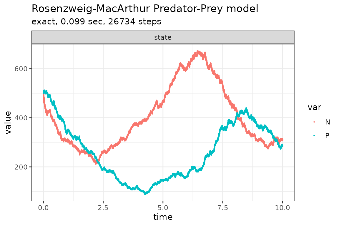
Run simulations with the Exact method

set.seed(1)
out <- ssa(
  initial_state = initial_state,
  reactions = reactions,
  params = params,
  final_time = final_time,
  method = ssa_exact(),
  sim_name = sim_name
) 
plot_ssa(out)

## Loading required namespace: ggplot2

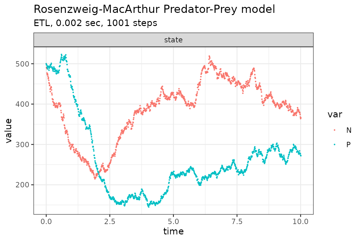
Run simulations with the Explict tau-leap method

set.seed(1)
out <- ssa(
  initial_state = initial_state,
  reactions = reactions,
  params = params,
  final_time = final_time,
  method = ssa_etl(tau = .01),
  sim_name = sim_name
) 
plot_ssa(out)

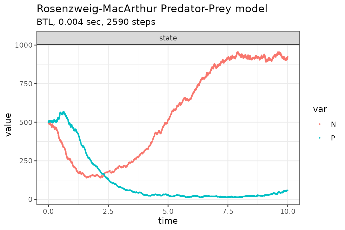
Run simulations with the Binomial tau-leap method

set.seed(1)
out <- ssa(
  initial_state = initial_state,
  reactions = reactions,
  params = params,
  final_time = final_time,
  method = ssa_btl(),
  sim_name = sim_name
) 
plot_ssa(out)

References

Pineda-Krch, Mario, Hendrik J. Blok, Ulf Dieckmann, and Michael Doebeli. 2007. “A Tale of Two Cycles – Distinguishing Quasi-Cycles and Limit Cycles in Finite Predator–Prey Populations.” Oikos 116 (1): 53–64. https://doi.org/https://doi.org/10.1111/j.2006.0030-1299.14940.x.