SIRS metapopulation model

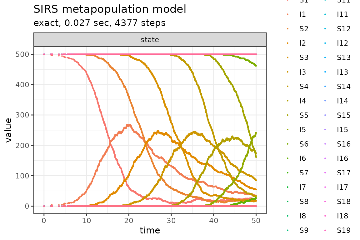
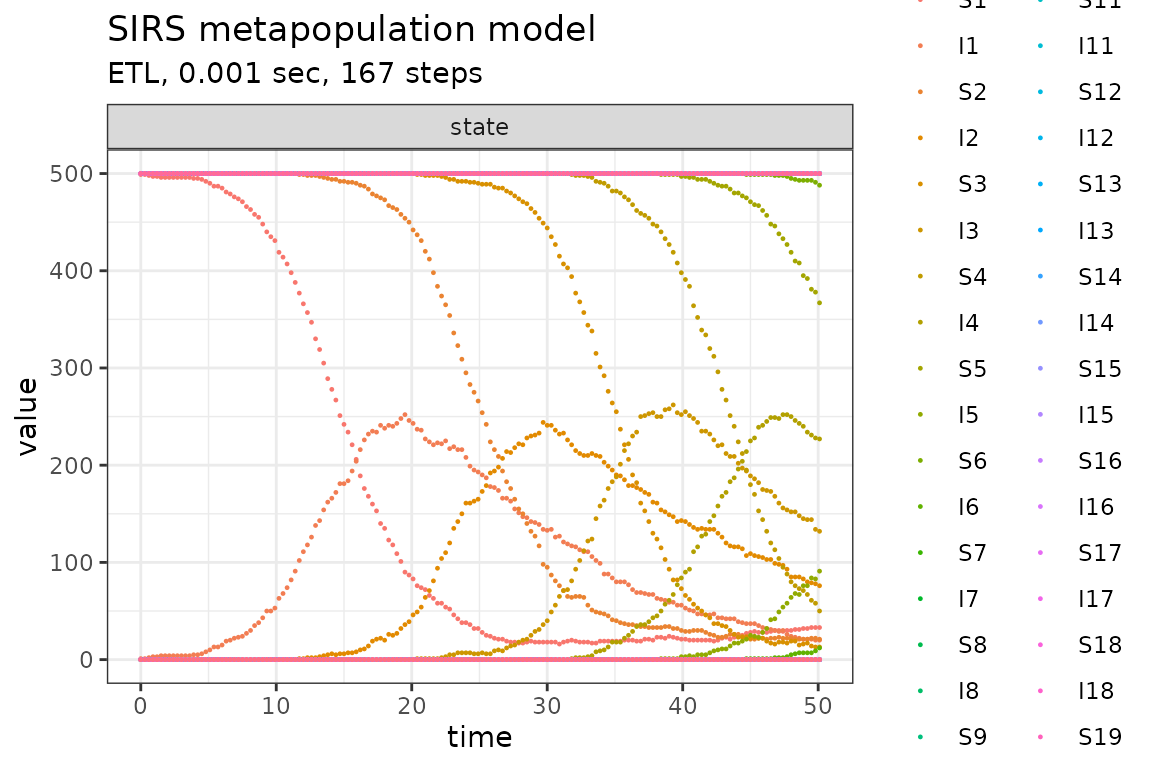
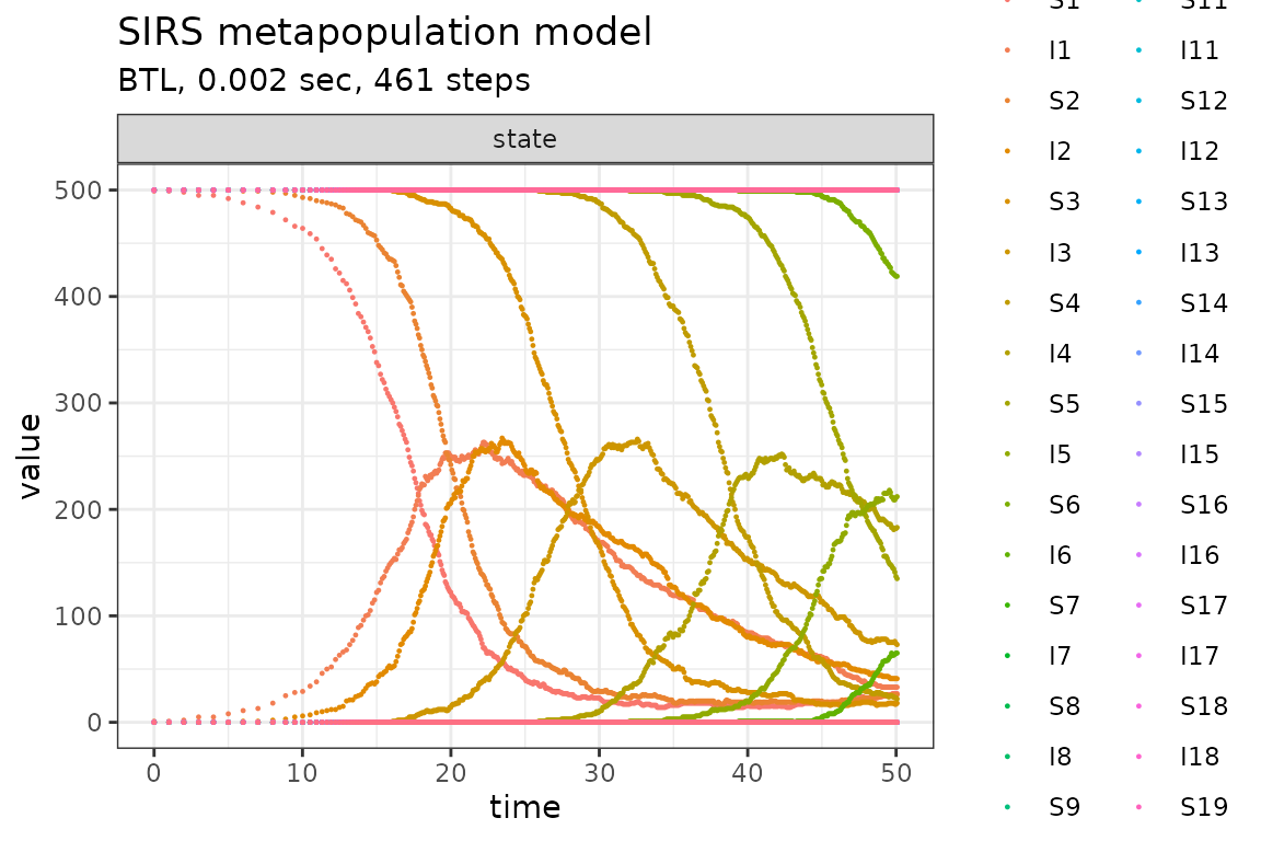
The SIRS epidemiological metapopulation model as defined by Pineda-Krch (2008).

Define parameters

library(GillespieSSA2)
sim_name <- "SIRS metapopulation model"
patchPopSize <- 500                    # Patch size
U <- 20                                # Number of patches
final_time <- 50                       # Final time

params <- c(
  beta = 0.001,                        # Transmission rate
  gamma = 0.1,                         # Recovery rate
  rho = 0.005,                         # Loss of immunity rate
  epsilon = 0.01,                      # Proportion inter-patch transmissions
  N = patchPopSize                     # Patch population size (constant)
) 

Create the named initial state vector for the U-patch system. The structure of initial_state is as follows (assuming a patchsize of 500 individuals),

initial_state <- c(
  S1 = 499, I1 = 1, 
  S2 = 500, I2 = 0,
  S3 = 500, I3 = 0, 
  ... 
  S20 = 500, I20 = 0
)

initial_state <- c(patchPopSize - 1, 1, rep(c(patchPopSize, 0), U - 1))
names(initial_state) <- unlist(lapply(seq_len(U), function(i) paste0(c("S", "I"), i)))

Define the state change matrix for a single patch

reactions <- unlist(lapply(
  seq_len(U),
  function(patch) {
    i <- patch
    j <- if (patch == 1) U else patch - 1
    
    Si <- paste0("S", i)
    Ii <- paste0("I", i)
    Ij <- paste0("I", j)
    list(
      reaction(
        propensity = paste0("(1 - epsilon) * beta * ", Si, " * ", Ii), 
        effect = setNames(c(-1, +1), c(Si, Ii)),
        name = paste0("intra_patch_infection_", i)
      ),
      reaction(
        propensity = paste0("epsilon * beta * ", Si, " * ", Ij),
        effect = setNames(c(-1, +1), c(Si, Ii)),
        name = paste0("inter_patch_infection_", i)
      ), 
      reaction(
        propensity = paste0("gamma * ", Ii),
        effect = setNames(-1, Ii),
        name = paste0("recovery_from_infection_", i)
      ),
      reaction(
        propensity = paste0("rho * (N - ", Si, " - ", Ii, ")"),
        effect = setNames(+1, Si),
        name = paste0("loss_of_immunity_", i)
      )
    )
  }
), recursive = FALSE)

Run simulations with the Exact method

set.seed(1)
out <- ssa(
  initial_state = initial_state,
  reactions = reactions,
  params = params,
  final_time = final_time,
  method = ssa_exact(),
  sim_name = sim_name
) 
plot_ssa(out)

## Loading required namespace: ggplot2

Run simulations with the Explict tau-leap method

set.seed(1)
out <- ssa(
  initial_state = initial_state,
  reactions = reactions,
  params = params,
  final_time = final_time,
  method = ssa_etl(),
  sim_name = sim_name
) 
plot_ssa(out)

Run simulations with the Binomial tau-leap method

set.seed(1)
out <- ssa(
  initial_state = initial_state,
  reactions = reactions,
  params = params,
  final_time = final_time,
  method = ssa_btl(),
  sim_name = sim_name
) 
plot_ssa(out)

References

Pineda-Krch, Mario. 2008. “GillespieSSA: Implementing the Stochastic Simulation Algorithm in r.” Journal of Statistical Software 25 (12). https://doi.org/10.18637/jss.v025.i12.